Blog: What the new VDA-AIAG SPC manual’s capability indices mean in practice: Cp, Cpk, Pp, Ppk, Cw, Cwk, Pm.G, Pmk.G, Cp.G, Cpk.G, Pp.G, Ppk.G

Introduction

In July 2026, the new VDA-AIAG SPC manual was released (VDA is the German Verband der Automobilindusrie and AIAG is the North American Automotive Industry Action Group). Amongst many other features, an important new item in this manual is the introduction of several new capability indices.

The new manual clearly states the manual is a recommendation and it will depend on the OEMs (Original Equipment Manufacturers) how far this is going to be a requirement. In this blog we will clarify these new indices, why they are proposed in the SPC (Statistical Process Control) manual and what the consequences in practice will be using these new indices.

Definition of Current Capability Indices

History

What is important to know before we will explain the definitions of the indices is that the definitions in the past have changed. Ppk was defined under the Q101 system of Ford as the preliminary capability index and the Cpk was defined as the long-term capability index.

In some cases the Cpk value on the histogram was calculated differently from the Cpk calculations on the control chart. When the big three (Ford, GM and Chrysler) merged their quality manuals into the QS9000 system the definitions were changed and these definitions are still the standard nowadays in the IATF16949 manual. It is also important to understand that these definitions are the standard in the Aerospace Industry. For example, these definitions are used in the RM13006 manual.

The definition of indices used until now were as follows:

Cp

Cp (sometimes also named Cpi) stands for the capability index of the process. The formula for the calculation is:

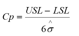
The  refers to the estimated standard deviation. The estimated standard deviation is calculated using the following formula:

 where

is the average range of subgroups and

is taken from a statistical table.

Cpk

Because the Cp index alone doesn’t indicate if you are producing within specifications, we need an indication whether the process is centered between the specification limits or not. Therefore the Cpk index is used. The formula is:

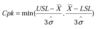
So if the process is exactly in the middle of the LSL and USL (the Lower and Upper Specification Limit), the Cp and Cpk index are the same.

If we now report both Cp and Cpk index, we know how capable the process is to produce within the required variation (tolerance) and if the process is producing in the middle of the tolerance.

Pp

Is the information about Cp and Cpk enough to indicate if the process is running within specification?

The answer is no because these 2 indices are calculated based on the within-subgroup variation and it is still possible there is a large amount of between-subgroup variation which is not taken into account. Let me try to explain this with an example.

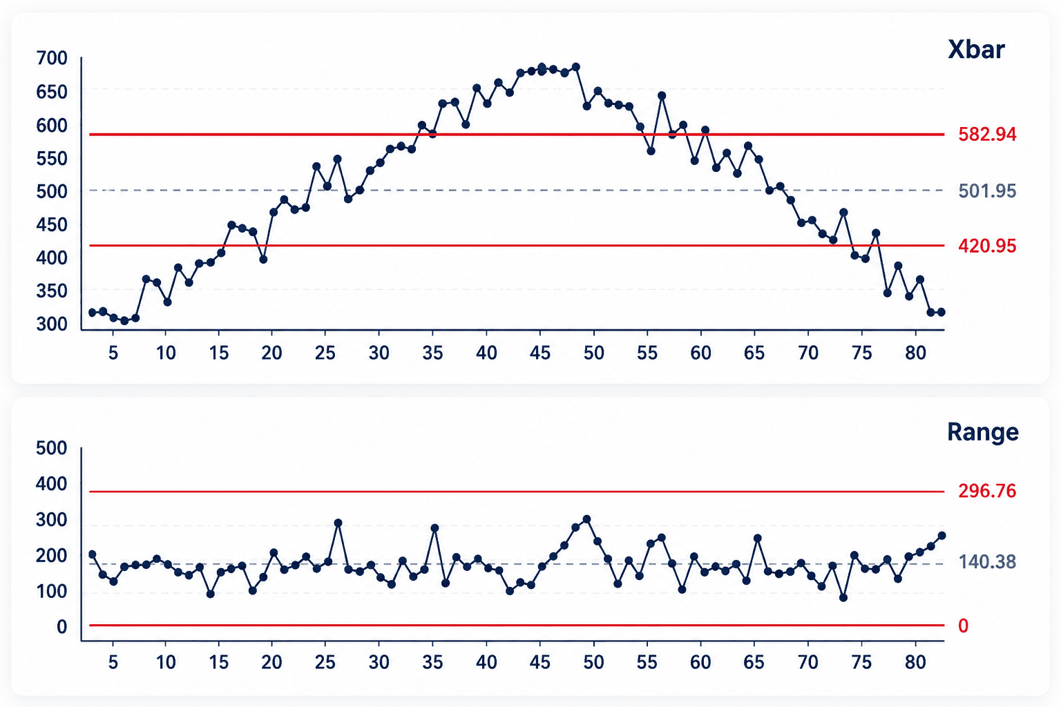
Figure 1: Control Chart from simulated data in Datalyzer SPC

The chart in Figure 1 shows a process where we had a lot of variation between subgroups (Xbar chart), but the variation within the subgroup was in control (Range chart).

The Cp index for this process is 1.64 and the Cpk index for this process is 1.62, which indicates the process is capable to produce within the required variation and over the reported time period this process is in the middle of the tolerance. For this same process, however, the Pp and Ppk indices are much lower (Pp = 0.90 and Ppk = 0.88), because they also include the large between-subgroup variation that is clearly visible in the Xbar chart but is invisible to Cp and Cpk.

We see that these 2 indices are not enough and we need more information to know if the process is producing within specification limits. If we only use Cp and Cpk we need to add the requirement that the process must be in control. If the average chart is in control it indicates the process is stable and the process average is not fluctuating.

However, we don’t always have the chart available when analyzing process data, for example if we report a large number of characteristics. In that case we could indicate the percentage of subgroups out of control but there is also another possibility.

We can also know if the process is stable by calculating the Process Performance Index Pp. The Pp index is calculated in the same way as the Cp index but now using the real standard deviation instead of the estimated standard deviation. So the formula is:

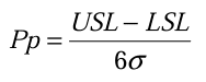
So the Pp index uses both within-subgroup variation and between-subgroup variation in the calculation and indicates how well the process was capable to produce within specification limits over the reported time period. The Ppk index is calculated in a similar way as the Cpk index and needs no further explanation.

Read our other blog for more information about the current four main Capability Indices: Capabilities Explained.

Potential problems with the use of the current indices

The capability indices assume the data is following a normal distribution. In the majority of situations in industry that is a fair assumption. But in some specific cases the data is not normally distributed. Examples are flatness, perpendicularity, position of a hole, tensile strength tests, etc. Some of them have a natural limit, some of them are skewed. In that case we need to use a non-normal capability analysis where we have to do the following analysis on the data:

Establish the best-fit distribution of the data.

Based on the selected distribution calculate the 0.135%, 50% and 99.865% quantiles.

Now calculate the capabilities based on the quantiles instead of using the sigma values.

Non-normal capability is not new. Datalyzer has already been offering Non-normal capability with distribution fitting in the Datalyzer SPC software for more than 30 years.

What is new in the VDA-AIAG SPC manual is that they recommend not to use the sigma method at all anymore and always use distribution fitting. In case the data best fits a normal distribution the results will be the same. Let’s provide an example to get an idea of how big the impact is.

We used AI to generate 3 different non-normal distributions of 125 measurements and imported them in Datalyzer Qualis SPC. A slightly skewed data set (folded normal c=0.5), a moderately skewed data set (folded normal c=2.0) and a heavily skewed data set (lognormal)

Below you see the 3 distributions.

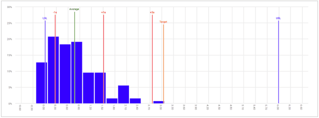
Figure 2: Slightly skewed data set

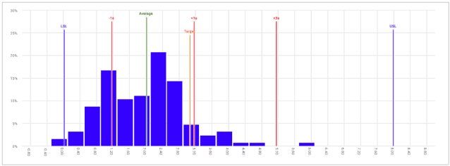
Figure 3: Folded normal moderately skewed data set

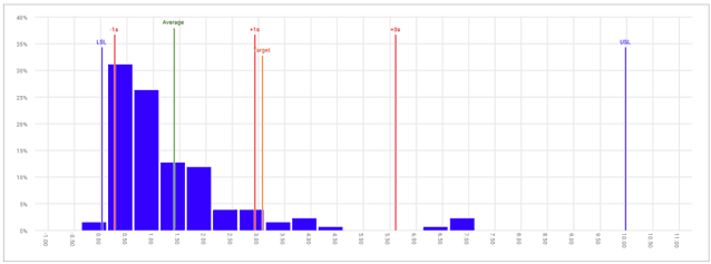
Figure 4: Heavily skewed dataset (lognormal)

In practice, we often see that these skewed distributions only have 1 active specification. We see an LSL of 0 where we cannot go below (flatness, perpendicularity, etc.) or we have no USL, for example tensile strength. Because we did not take subgroups we will only compare the Ppk values with Non-Normal capability calculations. Because of the diferent type of distributions/ processes, it makes sense to review the Pp LSL, Pp USL, NCp LSL and NCp USL for these examples. Ppk and NCPk report the lowest value of the two indices (Pp/NCp-LSL versus Pp/NCp USL) In the following table you see the results of the calculations.

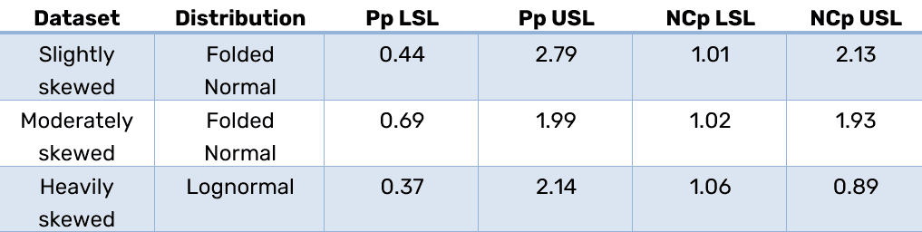
In case you have a natural limit of 0 where you cannot go below, the Ppk will be equal to Pp USL or NCp USL. The lower side is not evaluated here because 0 is a physical boundary rather than a real specification limit, so only the upper specification limit determines the capability. You see in the table that the non-normal capability will be lower than the regular capability based on the normal distribution.

In case you have no upper limit like with tensile strength, you see that the non-normal capabilities are better than the regular Ppk. It shows that in cases of heavily skewed distributions it will make a difference.

In the example above, we used a specific distribution to generate the data. In real life it becomes a bit more complex. We do not know the distribution so we have to do goodness-of-fit tests to establish the distribution. When we apply that in the example above, the goodness-of-fit test was even recommending a different type of distribution than what was used to generate the data. So when applying a goodness-of-fit test, you need to analyze the data and based on engineering knowledge you need to select the best distribution for your data. A goodness-of-fit test might recommend a folded normal distribution, but you might have a normal distribution with some out of control subgroups, so based on engineering knowledge it might be that a different distribution should be used.

AIAG-VDA SPC Manual New Indices

The first change in the new manual is that a new index is introduced which is the Cw and the Cwk value. This capability value is exactly the same as the traditional Cp and Cpk value; the new name simply makes explicit that this is the within-subgroup value, so it can be distinguished from the new .G indices. The calculations are the same and the w stands for within-subgroup variation.

Six more new indices are introduced which are according to ISO22514 and ISO3534:

Pm.G, Pmk.G, Cp.G, Cpk.G, Pp.G, Ppk.G.

There are similar indices introduced based on Z values, but we will leave it out of scope because they will hardly be used in practice. The calculation of all the six mentioned indices is the same and according to ISO. The suffix .G means the index is calculated from the distribution quantiles (the geometric method), instead of from the sigma value; this is why these six are also called the geometric capability indices.

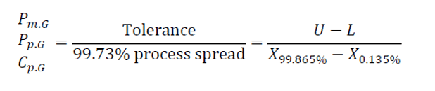
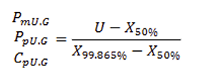
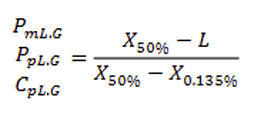
Where ‘L’ and ‘U’ refer to the LSL and USL limit (the customer specificatoin limits).

The idea is that you can only use Cp.G and Cpk.G in case you have a stable process which is in control. Now 3 phases are identified. During release of the machine, you should use Pm.G and Pmk.G. You take 50 consecutive samples from a machine without changing anything.

During prelaunch, you can do a process capability study and then you use Pp.G and Ppk.G. During prelaunch, you do not know all potential special causes yet so you cannot use Cp.G and Cpk.G. During steady production, you can use Cp.G, Cpk.G, Pp.G and Ppk.G.

The good thing about this approach is that it clearly describes the logic of how to apply SPC in the different phases — something which was mostly already done in practice for 30 years but was not clearly defined in the old SPC manual. The bad thing about this new approach is that it will generate a lot of confusion.

A process is defined as stable if no subgroup falls outside the control limits — or, if you apply extra rules such as runs and trends, if no rule violation is found on the chart. If you analyze one chart for a week with 100 subgroups, you might find no out of control subgroups but that is not how it works in real life.

An example: One of our customers measures 2500 characteristics on each product during a CMM (Coordinate Measuring Machine) study. The false alarm rate with 3 sigma limits is each 370 subgroups for individuals and approx. each 100 subgroups for the moving range.

If we use an ImR (Individuals and moving Range) chart to record all measurements and we use the normal 3-sigma limits, we would have a false alarm every 80 characteristics if we would deactivate all special alerts. In that case in one CMM measurement we would have 31 false alarms. If we report during production about 125 parts supplied, we would have 3875 false alarms. Processes are never completely stable, so in practice there would be much more alerts.

Note: The new VDA-AIAG manual indicates a different way of calculating limits based on an alpha risk which reduces false alarms for limits if you take an alpha level of 99.99%. But that has serious efficiency consequences setting up the charts and there are much easier and smarter ways to handle this. We will discuss this in a different blog.

Here our practical recommendation departs from a literal reading of the manual: in practice it doesn’t make sense to use Cp.G and Cpk.G unless you are only discussing and analyzing 1 characteristic. To show if a process is stable it is easier to report about Cw, Cwk and Ppk.G. If Cwk and Ppk.G are more or less similar, the process is stable. If not, it might still be stable and could be heavily skewed.

Changes in Datalyzer Qualis 4.0 SPC Software and Recommendations

In Datalyzer we need to keep Cp, Cpk, Pp and Ppk according to the existing definitions because those are used in several other industries than Automotive. Many suppliers active in Automotive Industry also need to report to Aerospace, Defense, Medical Devices, Food and other industries where the normal Cpk and Ppk definitions are used.

Datalyzer will implement the new indices besides the traditional indices. We can already define per characteristic what indices should be used in reporting. Based on a preference setting, the existing NCp and NCpk index can be renamed to the new definition and add a new Cw index.

We already monitor full tracking and tracing so while reporting we can easily identify if it is a machine study, a process capability study or full production even if charts have a mixture of existing products and new products or a change of a product where a new PPAP (Production Part Approval Process) is required.

We will recommend companies to clearly use the addition .G if a non-normal capability is used to avoid confusion between normal Cpk and Ppk and the geometric capabilities. We would recommend never to use Cp.G and Cpk.G unless in a single analysis of a chart because there will be a lot of confusion about the interpretation.

Reach out to Datalyzer in case you have comments or would like to see how this would work in your organization.