50+ countries
Global use, local impact

47 years in business
Originated in 1979

50+ employees
Europe, USA and Asia

2000+ customers
More than 20.000 users
Modernizing your Gage R&R Studies with Qualis 4.0 MSA Gage Management
Introduction in Gage Repeatability and Reproducabililty
Measurement System Analysis (MSA) is a fundamental aspect of quality management, ensuring the reliability and accuracy of measurement systems in various industries. Among the most widely used MSA techniques is Gage Repeatability and Reproducibility (GR&R) analysis, whichevaluates the precision and consistency of measurement systems through systematic studies.
GR&R studies are essential for identifying and mitigating sources of measurement error, enabling organizations to make informed decisions and enhance product quality and process efficiency. However, conducting GR&R studies traditionally involves complex calculations, tedious data management, and a significant investment of time and resources. To address these challenges and streamline the GR&R process, we, the Datalyzer team, have developed Qualis 4.0 MSA Gage Management as a state-of-the-art MSA software solution.
Using Qualis 4.0 MSA Gage Management for GR&R Studies
Nowadays, GR&R studies are conducted using three primary types: Type 1, Type 2, and Type 3 GR&R Study. Each type offers distinct methodologies and approaches for analyzing measurement system variability, allowing organizations to tailor their assessments to specific requirements and objectives. These types of GR&R studies play a vital role in enhancing product quality, optimizing manufacturing processes and driving continuous improvement initiatives.
Type 1 Gage R&R Study
Type 1 GR&R Study is typically used to assess and understand the variation that is coming from the gage/ equipment itself only. In many organizations, the type 1 study is even a prerequisite before doing a complete variable Measurement System Analysis (MSA) study. A Type 1 GR&R Study requires one operator to measure one part for at least 25 to 50 times. This operator must know the part’s reference value as well.As only one operator (appraiser) is involved, there will not be any appraiser influence in a Type 1 study. In another words, there will be no ‘Reproducibility’ factor in this study and the focus lies on the ‘Repeatability’ factor of the gage. Since one of the objectives of Type 1 study is to assess gage repeatability, the concept is to evaluate whether the gage measurement variation is not too large compared to the part’s tolerance. To do this, it is preferred to choose the part’s characteristics with two-sided specification limits in order to establish a tolerance range.
Few metrics are typically used to evaluate the gage repeatability namely:
- Cg
- Cgk
- % EV (Repeatability)
- % EV (Repeatability and Bias)
Cg is a gage capability metric that compares the gage study variation (the spread of the 25-50 measurement data) to the part tolerance. Generally, a threshold limit of 1.33 is used for Cg. If Cg is higher than 1.33, the gage measurement variation is smaller compared to the tolerance range.
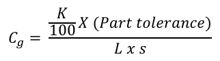
Above is the formula for Cg where K is the percentage from the part tolerance (In Datalyzer we set this at default 20) while L is number of standard deviations that represents entire process by default 6 (infamously known as six sigma). Part tolerance is USL-LSL while s is the standard deviation from the 25-50 measurements.
Cgk is a metric that not only compares the gage study variation to the part tolerance (similar to Cg) but it also checks whether the measurements are on the exact target reference value of the part. Following is the Cgk formula:
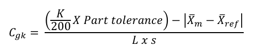
Where K is percentage from part tolerance (default 20), L is number of standard deviations that represents half of process spread (typically 3 is used as L), Xm is average of 25-50 measurements while Xref is the reference value of the part.
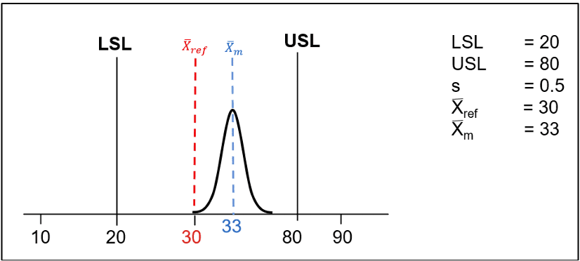
The further the average of the measurements are from reference value, the higher the “bias” of the gage is. The term bias here referring to the distance between Xm and Xref. In above image Cgk equals to 2. If Cgk higher than 1.33, that means the gage measurement standard deviation is narrower compare to the part tolerance and at the same time, the bias of the gage compares to the reference value is not significant.
In a Type 1 Study, apart from Cg and Cgk, two alternative metrics that evaluates gage repeatability are %EV (repeatability) and %EV (repeatability and bias). The two terminologies have threshold limits commonly set as 15%. If %EV (repeatability) higher than 15%, the measurement variation is larger/wider compared to the part’s tolerance. Basically %EV is the reciproke of Cg. The formula is:

%EV is 20/Cg. If Cg = 1.33 then %EV will be 15%.
If the %EV (Repeatability and Bias) is higher than 15%, the measurement variation is larger than the part tolerance and at the same time, the bias (difference between average Xm and Xref) is significant. Note that commonly 10 or 15% is used as threshold limit where ideally lower than the threshold percentage is desired.
From above four metrics (Cg, Cgk, %EV Repeatability and %EV Repeatability and Bias), it can be observed that the gage bias towards the refences is also frequently considered and checked. Therefore, it is common to include a 1 sample T-test in Type 1 GR&R studies to further strengthen the statistical significance whether the Xm is different/ far away from Xref. To evaluate using a 1 sample T-test, the associated p-value needs to be higher than 0.05 to conclude that there is no significant difference between Xref and Xm.
In Datalyzer Qualis 4.0 MSA Gage Management, between 25 to 50 parts can be selected to perform a Type-1 Gage Study. When the reference value, lower specification limit (LSL) and upper specification limit (USL) are added, the summarized information will be shown in the ‘Dataset’ tab as below.
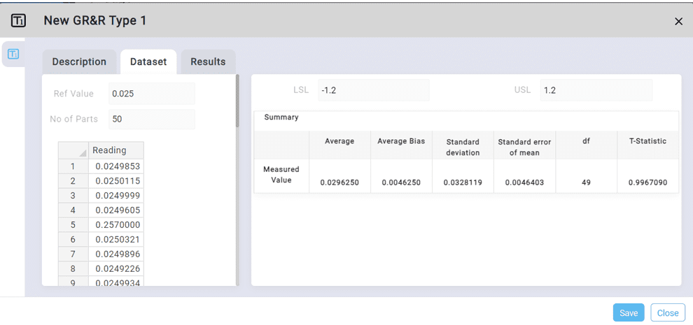
The judgement will be shown in the ‘Results’ tab where the mentioned criteria metrics will be used. The below study results show a ‘Pass’ judgement for Type 1 GR&R Study as p-value is higher than 0.05, Cg and Cgk are higher than 1.33, and both %EV are less than 10%.

Some organizations only use the p-value for the Type 1 Gage Study, while other organizations uses only Cg/Cgk. Any choice of criteria can be configured as default rule for your company in Datalyzer Qualis 4.0 MSA Gage Management software.
Judgement Criteria:
Different criteria are used in different industries, so this might be confusing for end users. %EV (Repeatability and Bias) is not the same as %EV in GRR Type 2 studies because Bias is not included in a Type 2 study. So the criteria might even be different per type of study. Also customers might require other criteria.
For example, for Type 2 studies in the AIAG (Automotive) manual the requirement for GR&R is: GRR < 10% is good, 10% < GRR < 30% is marginal andGRR > 30% is bad.
Minitab uses 2 criteria: GRR < 15% is good and GRR > 15% is bad. For Cg and Cgk we will use corresponding criteria. In Datalyzer we by default offer the same criteria as AIAG but the end customer will be able to change the criteria if they want to deviate from the automotive standard.
Type 2 Gage R&R Study
The Type 2 Gage R&R study is the most applied GR&R method in organizations that apply MSA studies. There are three approaches or methods to evaluate the results of a Type 2 GR&R Study which are:
- Range Method
- Average and Range Method
- ANOVA Method
In Datalyzer Qualis 4.0 MSA Gage Management, we support all three methods.
Range Method (also known as ‘Short Study’ or ‘Short Form’) is a simplified variable GR&R method and it is not to be used to evaluate a full measurement system entirely from its results. It is often used as a quick approximation of the measurement variation and to detect any major changes in GR&R for existing gages.
The Range Method often uses 2 appraisers and 5 parts where each appraiser will measure once (one trial). From the results the %GRR will be calculated where:
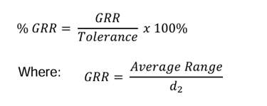
The GRR will be calculated from the average of each range divided by the constant d2 that is obtained from statistical constant tables. From %GRR, we can interpret the proportion of measurement variation compared to the total variation. The measurement variation cannot be too large compared to the total variation.
In Datalyzer Qualis Gage Management, the GR&R Type 2 Study will provide a ‘Study Type’ option where the user can choose ‘Short Study’ followed by ‘Range Method’ in the ‘Calculation Method’ field to opt for the Range Method in GR&R Study.

The results will appear after the data entry where the typical criteria of the study will be evaluated depending on %GRR. Ideally %GRR needs to be less than 10% for the Range Method Study to be considered passed.

The second method in Type 2 GR&R Study is known as Average and Range Method. In this study, typically 2 to 3 appraisers will measure between 10 to 35 parts with 2 to 4 trials for each appraiser. In Datalyzer Qualis Gage Management, multiple methods can be used to calculate total variation. In below example ‘Study Variation’ is chosen.

There are three methods to obtain Total Variation in a GR&R Study:
1. From the total Study Variation, taken from the GR&R measurement data itself:

2. From Statistical Process Control (SPC), taken from standard deviation in SPC from a stable process.

3. From total Tolerance of the process, USL and LSL.

Datalyzer supports all above methods in obtaining the Total Variation in GR&R Study. In Datalyzer Qualis 4.0 MSA Gage Management software if the user enables the “SPC” checkbox shown below, the user can select a part and characteristic from the SPC system and the Qualis Gage Management software will automatically import the latest process variation and process tolerance (LSL and USL) from the Datalyzer SPC Software.
The MSA requirement that the variation in parts selected for the study should be representative for the process is not always easy to fulfill. Therefore we offer the option to take the real process variation to make sure this requirement is always met.

Using the Average and Range method, the results can be viewed in the Results tab as shown below:

The Judgment Criteria for a Type 2 GR&R Study are based on %GRR (percentage of Gage Repeatability and Reproducibility) and ndc (number of distinct categories). For the Type 2 Study to be considered Passed, %GRR needs to be less than 10%, and ndc needs to be equal or higher than 5.
%GRR in Average and Range depends on either equipment variation (EV) or Appraiser Variation (AV). If %GRR is higher than 10%, the Type 2 Study is marginal or fails and the user can view EV and AV to find the factor most contributing to the failure.
Another criteria which determines the success of Type 2 Study is ndc. Ndc stands for number of distinct categories. Ndc is often used to identify a measurement system’s ability to detect a difference in the measured characteristic. Various industries uses the common approach of ndc stated by Wheeler,1989 where ndc can be estimated using formula:
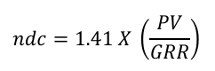
Then the ndc is cut off to a full number. So ndc of 5.67 will be a ndc of 5.
Aside from numerical calculations, Datalyzer Qualis Gage Management software also offers Graphical Visualization to help users in providing more information on the GR&R Study. Following graph plots are available in the Type 2 Average and Range Method:
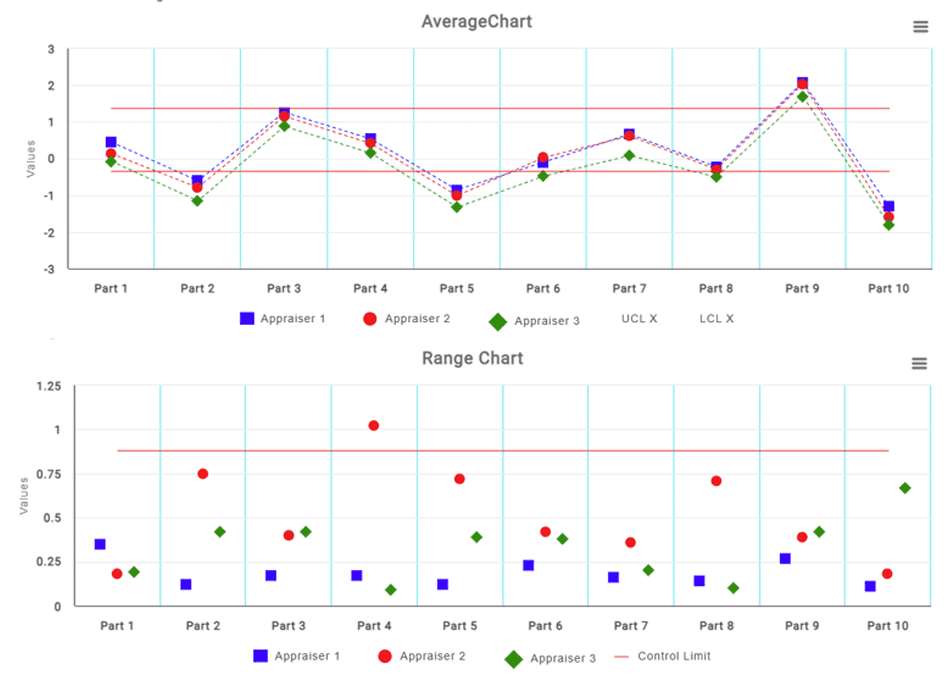
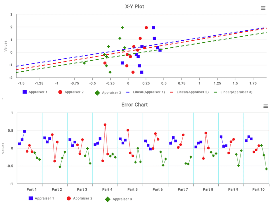
The third method in Type 2 GR&R Study is the ANOVA (Analysis of Variance) Method. The same measurement data that is used in the Average and Range Method can be used in the ANOVA method as well but the calculation methods are different.
In the Average and Range Method, the calculation components are divided only between Equipment Variation (EV) and Appraiser Variation (AV). In ANOVA, it also considers the interaction between appraisers and the parts which is why ANOVA is often more preferred compared to the Average and Range method. The following example below explains about the interaction between appraisers and parts.
In an automotive manufacturing plant, two operators, Sarah and Mike, are responsible for inspecting the dimensions of engine valves. The goal is to assess the variability in measurements between the operators.
Scenario 1: If Sarah consistently measures engine valves larger than Mike, regardless of the product measured, there may be a main effect of appraisers. Above scenario 1 can be detected both in ANOVA and Average and Range Method.
Scenario 2: However, if the difference in measurements between Sarah and Mike varies significantly depending on whether they are inspecting specific valves there is likely an interaction effect. Above scenario 2 can be easily detected in the ANOVA method as ANOVA considers the interaction between factors, in this case between Sarah/Mike and specific engine valves.
In Datalyzer Qualis 4.0 MSA Gage Management software, the ANOVA calculation method can be selected if preferred.
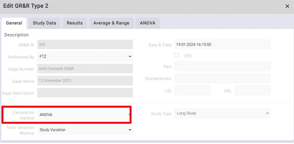
Upon entering the measurement data, the ANOVA supporting calculations can be seen in the example below.
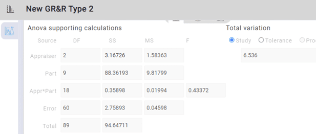
Above supporting calculations can give some information for users based on DF (degree of freedom), SS (Sum of Squares), MS (Mean of Squares) and F-statistic.
In GR&R ANOVA, Degrees of freedom (DF) represent the number of independent pieces of information available to estimate variability in the measurement system. Specifically:
1. Between-Operator Degrees of Freedom: This represents the degrees of freedom associated with differences between the operators (appraisers) in their measurements. It is equal to the number of operators minus one.2. Within-Operator Degrees of Freedom: This represents the degrees of freedom associated with differences within each operator’s measurements. It is equal to the total number of measurements minus the total number of operators.
Mean square (MS) represents the average variability within and between operators. Specifically:
1. Mean Square Between Operators: This represents the average variability between operators and is calculated by dividing the sum of squares between operators by the degrees of freedom between operators.2. Mean Square Within Operators: This represents the average variability within each operator’s measurements and is calculated by dividing the sum of squares within operators by the degrees of freedom within operators.
Sum of squares (SS) represents the total variability in the measurement system, which is partitioned into variability between operators and variability within operators. Specifically:
1. Sum of Squares Between Operators: This represents the sum of squared deviations of operator means from the overall mean, weighted by the number of measurements for each operator2. Sum of Squares Within Operators: This represents the sum of squared deviations of individual measurements from their respective operator means.
The F-statistic is a ratio of two mean squares. A larger F-value indicates a greater difference between operators relative to the variation within operators, suggesting that the measurement system may not be reliable. Following screen will be shown for ANOVA Results for a Type 2 GR&R Study:
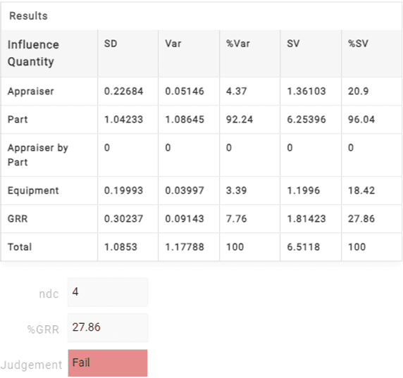
For the above results, the user can see similar criteria as for the Average and Range method which is %GRR and ndc value. Above Type 2 Study fails due to high %GRR (higher than 10) and low ndc value (lower than 5). User can also opt to look for %GRR at the above table manually at the last column (%SV) which is % Study Variation column.
Type 3 Gage R&R Study
The Type 3 Gage R&R Study is a modified version of a Type 2 Study where in this study, no operator influence exists. Type 3 is used in the industry for automated machines/ testers that have large number of characteristics without any significant human influence factor in its measurement system.
In Type 3 studies, typically 25 parts will be chosen to be measured twice (two trials) and no operator is involved so the results will be taken from one machine. In this case, machine is the appraiser itself.
In contrast with Type 1, Type 3 judgement criteria are the same as for Type 2 which is %GR&R whereas Type 1 looks into Cg/ Cgk and other criteria which emphasizes more on the Repeatability and Bias factor. The main difference in calculation between Type 3 and Type 2 Studies is the %GRR which is calculated purely based on Equipment Variation (EV) while Appraiser Variation (AV) is omitted from the GRR calculation. Which means in Type 3 studies, the formula for GRR is:

In Datalyzer Qualis Gage Management Software, both ANOVA and Average and Range can be selected for a Type 3 Study. After data entry, the result screen for the Type 3 Study will look similar to Type 2’s layout screen.

In Above example, ANOVA method is chosen in the Type 3 Study. Do take note the Appraiser factor and Interaction between appraiser and Parts will be omitted from the ANOVA table (shown as zero) due to no appraiser effects.
The screen above shows the results of the study of one characteristic. But in most cases we measure hundreds of characteristic (eg CMM of complex parts or electrical testing of a PCB board). In that case, Datalyzer MSA Gage Management software can be used in combination with the automatic import module to import all the characteristics at once and present a full MSA study of hundreds of characteristics. Currently most companies are only making a selection of the most critical characteristics because it is too time consuming to perform studies for hundreds of characteristics. By completely automating this process you get an immediate indication which characteristics might be critical based on MSA results.
9%
Cost Reduction Achieved by customers


What customers say
“Datalyzer helped us automatically link quality data from all processes for advanced analysis”
Dave Beeren
Yield Engineer, Philips
Industries we serve

ISO Certified
ISO 27001 & SOC2