Blog: How to use Design of Experiments (DOE) in Datalyzer Qualis 4.0 Analytics

Concepts and Strategies of DOE

DOE is not limited to a single type of experimental design. The appropriate approach depends on the objective of the experiment and the level of process knowledge available. Common objectives include comparison, screening, characterization, optimization, and robust design. In practical applications, DOE is often conducted as a sequential strategy based on above objectives rather than as one large experiment.

The stages of Design of Experiments (DOE)

1. Preparation & Design Stage (Experiment Setup)

During the preparation stage of Design of Experiments (DOE), the experimental design is established and the design matrix is created. This stage determines how the experiment will be structured before any experimental data are collected.

While preparing the DOE, the Factors are defined as well as their levels. Factors are the input variables that are deliberately changed during the experiment to determine their effects on the response. Factors may represent process parameters, material characteristics, equipment settings, environmental conditions, or other controllable inputs. Factors may be classified as:

For a two-level factorial DOE, each factor is commonly represented by: -1 = low level and +1 = high level. The actual physical values remain important because they define the practical experimental conditions. After identifying the factors and their levels, an appropriate experimental design must be selected. For two-level factorial experiments, two important design options, both supportd in Datalyzer Qualis 4.0 Analytics are:

Once the design is selected, the Number of Experimental Runs will be determined and the Response Variables are defined.

The Response Variable is the output measured from each experimental run. The response should directly represent the performance characteristic being investigated. Examples include: Product strength, Yield, Surface roughness, Dimensional accuracy, Cycle time, Defect Rate etc. Multiple responses may be included in the same DOE when the experiment is intended to study several performance characteristics simultaneously.

Before generating the final design matrix, decisions about how to handle center points, blocks, and replication are required. These decisions should be made during the design stage rather than after the experimental data have been collected. Then, code levels and run randomization can be defined and the design matrix can be created.

The final design should contain sufficient information for the experiment to be conducted consistently and traceably. The final design matrix should normally include: Experimental run number, Standard run number, Randomized run order, Factor names, factor coded values and actual values, response variables, Center-point identification, where applicable, Block identification, where applicable and  Replicate identification, where applicable.

Before proceeding to the experimental runs, the design should be checked to confirm that the experimental objective is clearly defined and that the responses are measurable and the required number of runs is feasible. The finalized design matrix then becomes the experimental plan for the subsequent data-collection stage.

Qualis 4.0 Analytics generates the Design Matrix based on the experimental design setup and configuration elements. Then, the actual experiment can be conducted according to the factor levels specified in the Design Matrix.

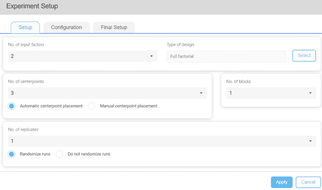
Figure 1: Example screen of Qualis 4.0 Analytics Experiment Setup – Setup

2. Data Collection and Validation

Once the experimental design and design matrix have been finalized, the experimental response data are collected according to the planned experimental runs. Before proceeding to process modelling, the collected response data should be assessed to determine whether they satisfy the basic statistical assumptions required for subsequent analysis. The three main characteristics considered are:

These checks provide an initial assessment of whether the collected data are suitable for subsequent statistical modelling. A typical interpretation is:

Check	Method	Desired Result
Randomness	Run test	p-value > 0.05
Randomness	Scatterplot + centerline	No systematic pattern
Normality	Probability plot	Points reasonably follow reference line
Normality	Normality test	p-value > 0.05
Equal Variance	Equal variance test	p-value > 0.05

These criteria should be treated as guidelines rather than automatic pass/fail rules. The p-value should be considered together with the corresponding graphical assessment and the practical behaviour of the data. If the data show no substantial evidence of non-randomness, non-normality, or unequal variance, the dataset can still be used in process modelling.

Once the experimental data have passed the initial validation checks, the next step is to use the DOE data to develop a mathematical model of the process.

In Qualis 4.0 Analytics, the experimental results are entered in the Response column of the DOE Design Matrix and the DOE is saved and the software will proceed to model optimization.

The modelling process does not begin by immediately deciding which factors are important. Instead, the experimental data are first used to construct an appropriate initial model containing the effects that can be estimated from the selected DOE. The initial model is then analyzed using regression and ANOVA to understand the contribution and statistical significance of the model terms. Where appropriate, the model is reduced by removing terms that do not provide sufficient evidence of contributing to the response. The reduced model is subsequently refitted and evaluated again until an appropriate final model is obtained. Qualis 4.0 Analytics DOE supports to re-fit the model and save the results.

The overall model significance is evaluated using ANOVA, which separates the total variation observed in the response into variation explained by the model and variation attributed to error. The ANOVA results also provide information about the individual model terms and the statistical evidence associated with each term.

The following example shows an ANOVA and model summary table containing the estimated coefficients, standard errors, degrees of freedom, adjusted sums of squares, adjusted mean squares, F-values, p-values, and model fit statistics.

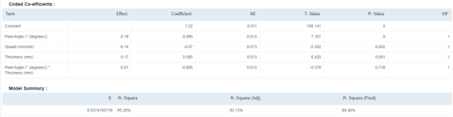
Figure 2: Model Summary DOE in Qualis Analytics

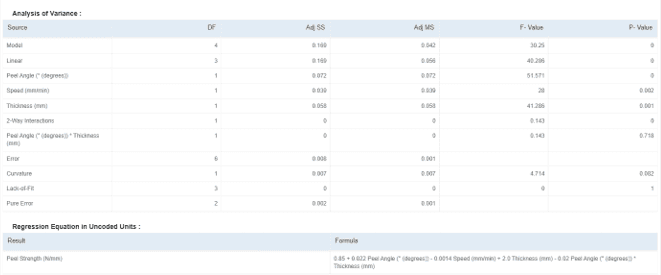
Figure 3: ANOVA and Regression Equation DOE in Qualis Analytics

The table provides several pieces of information that are used throughout model evaluation. The coefficient describes the estimated effect of a model term, while the standard error describes the uncertainty associated with that estimate. The degrees of freedom, adjusted sum of squares, and adjusted mean square describe the variation associated with each source. The F-value compares the variation associated with a term with the estimated error variation, and the corresponding p-value provides evidence for determining whether the term is statistically significant.

Before considering how much variation the model explains, the first question is whether the model as a whole provides sufficient statistical evidence that it explains a significant portion of the response variation. This is evaluated using the overall model ANOVA test. The interpretation at alpha level of 0.05 is:  p-value ≤ 0.05: the model is statistically significant. p-value > 0.05: insufficient evidence that the overall model is statistically significant.

A statistically significant model indicates that the variation explained by the model is sufficiently large relative to the experimental error to provide evidence that the model is useful for describing the response. However, establishing that the model is statistically significant does not tell us how much of the response variation is explained by the model or how well the model is expected to predict new observations. These aspects are evaluated by evaluating R2, Adjusted R2 , and Predicted R2, Lack of Fit and Residual Analysis.

The results from the preceding evaluations should be considered together to determine whether the reduced model is adequate for representing the process. The evaluation should consider:

These criteria should be considered together rather than relying on a single statistic. A high R2 , for example, does not automatically indicate an adequate model if the residuals show systematic patterns or significant lack of fit. If the overall evidence indicates that the model is adequate, the reduced model can be accepted as the final model and used for the next stage of DOE analysis.

3. Model Interpretation and Analysis (Model Analysis)

After the model has been evaluated and confirmed as adequate, the next step is to interpret the relationship between the factors and the response. The purpose of model interpretation is to understand how the factors affect the response, whether the effects are positive or negative, whether factors interact with one another, and how the response changes across the experimental region. The main tools used for interpretation are: Main Effects Plot, Interaction Plot, Contour Plot and Surface Plot.

Main Effects Plot

A main effects plot shows how the predicted or observed response changes as the level of one factor changes, while considering the response across the levels of the other factors. The general interpretation is based on the slope of the line.

The magnitude of the slope provides an indication of the strength of the main effect.

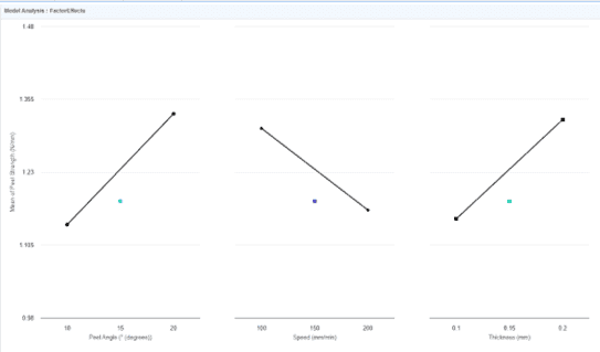
Figure 4: Main Effects Plot DOE in Qualis Analytics

Interaction Plot

An interaction plot is used to determine whether the effect of one factor depends on the level of another factor. Consider two factors, A and B. If the effect of A is approximately the same at both levels of B, there is little evidence of an interaction. If the effect of A changes depending on the level of B, an interaction may be present.

The plot can be interpreted using the relationship between the lines:

For example, if increasing temperature improves the response at low pressure but has little or negative effect at high pressure, temperature and pressure interact. The following example demonstrates the use of interaction plots to interpret the effects of the factors on the response.

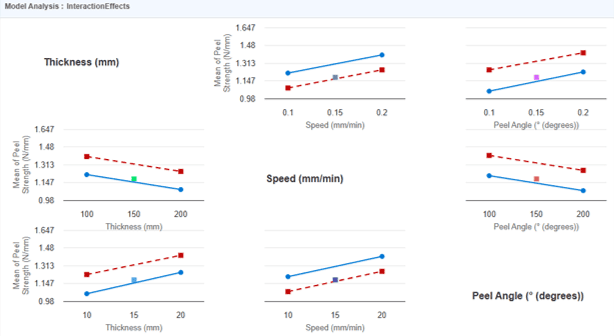
Figure 5: Interaction Plot DOE in Qualis Analytics

Contour Plot

A Contour Plot is a two-dimensional graphical representation used to visualize the relationship between a response variable and two input factors. It uses contour lines or shaded regions to represent areas with equal or similar response values. Similar to a topographic map, the contour plot helps users visualize the response surface and identify trends, peaks, valleys, and regions of interest.

In Qualis Analytics, select Contour Plot from the Plot Type field to generate a contour plot. Users can choose to generate All Plots or a Single Plot.

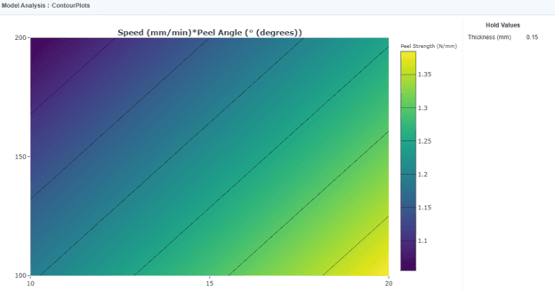
Figure 6: Contour Plot DOE in Qualis Analytics

Surface Plot

A surface plot provides a three-dimensional representation of the fitted response over two factors. The two factors are represented by the horizontal axes, while the predicted response is represented by the vertical axis. The resulting surface shows how the response changes as the two factors change simultaneously. The shape of the surface can provide information about: Direction of the response change, Strength of factor effects, Interaction between factors, Peaks and valleys and Curvature, where represented by the fitted model.

The surface plot therefore provides a visual interpretation of the mathematical model. The following example demonstrates how a surface plot can be used to visualize the response surface and the relationship between the factors.

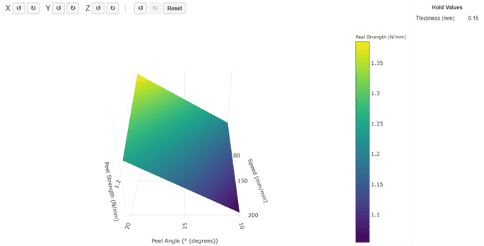
Figure 7: Surface Plot DOE in Qualis Analytics

4. Model Optimization and Prediction

After the model has been evaluated and interpreted, the final stage is to use the model to determine the desired factor settings, predict the expected response, and then confirm the prediction using an actual experiment.

Model Validation in Qualis 4.0 Analytics is used to determine the optimal factor settings based on the fitted model and the desired response. Users can select the type of optimization according to whether the response should achieve a specific target, be maximized, or be minimized. Three types of optimization are supported in Qualis 4.0 Analytics: 1. Target Response – determines the factor settings that achieve a desired target value for the response. 2. Maximize Response – determines the factor settings that maximize the response. 3. Minimize Response – determines the factor settings that minimize the response.

The result of model optimization are predicted factor/input to achieve the selected optimization objective. The Confidence Interval (95%) is also displayed to indicate the uncertainty associated with the model prediction.

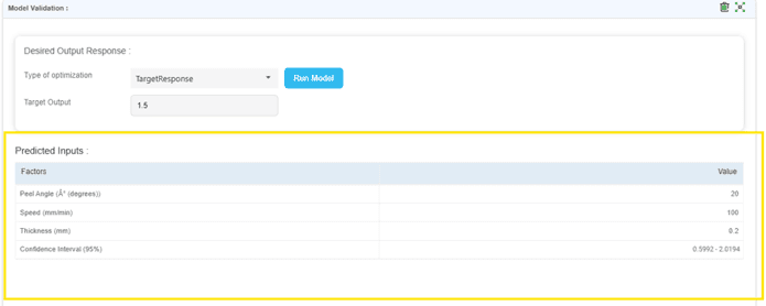
Figure 8: Model Optimization – Predicted Inputs – DOE in Qualis Analytics

It is advised to determine whether the actual process produces a response consistent with the model prediction by running a confirmation experiment using the final factor settings as presented in the Model Validation

The result should be interpreted in relation to the prediction uncertainty and expected process variation, rather than relying only on the percentage difference. If the actual result is reasonably consistent with the prediction and achieves the desired response objective, the model and selected operating conditions can be considered confirmed.

Final Comment

If you are interested to get started with DOE or looking for a tool to support your DOE experiments, or compare DOE with Machine Learning which is also available in Analytics then reach out to Datalyzer. Datalyzer supports customers providing Six Sigma training including DOE, and we provide additional documentation and information about the studies in the Qualis 4.0 Analytics User Manual.